This paper provides a thorough description of what a SeaSPY Overhauser magnetometer is, what it does, and how it does it. In doing so, it references advanced concepts in the fields of electromagnetics, quantum physics, and mathematics. However, it does not assume that its audience has a technical background, and its arguments are placed in language that anyone can understand.

Section 1 provides an introduction to the principles of magnetism. It describes how magnetic fields are modeled, and defines the terms necessary to understand the model. It also describes how different materials interact with magnetic fields, and how to detect objects using those interactions.

Section 2 introduces the Earth’s magnetic field, and gives an introduction to methods used to measure it.

Section 3 provides a thorough technical description of how a SeaSPY Overhauser magnetometer works.

Section 4 describes common terms and concepts that are used in magnetometry, and how they relate to the SeaSPY magnetometer.

Section 1: Modeling and Using Magnetic Fields

Vectors and Fields

The term vector refers to a quantity whose value may be represented by both a magnitude and a direction in space. Force, velocity, and acceleration are all examples of vectors.

A field may be defined mathematically as some function of a vector within a region of space, so that a vector quantity is defined at every point in the region. The field that is most familiar to us all is the gravitational force field generated by the Earth. We know this field exists because we can feel it all the time – our bodies have sensors that tell us it is all around us, wherever we go over the surface of the Earth.

Another field that is constantly present all around us is the Earth’s magnetic field. Although our bodies do not have sensors that allow us to detect this field directly, people have long had tools that can detect it and map it. A compass needle, for example, will have a force exerted upon it by a surrounding magnetic field; it is a tool that is designed to measure only the directional component of the magnetic field vector at its location.

In order to visualize a field that we cannot directly see, it is often necessary to make a map of the field, in the same way we map the Earth’s geography. One-dimensional maps chart the value of the field as it changes over a line of space. Two-dimensional maps are charts of the field over an area of space. A common model for a two-dimensional map is the contour map, which shows lines where the local vector is constant. The lines are spaced apart by the resolution of the map.

The Nature of Magnetic Fields

The symbol for magnetic field intensity is H, and its units are amperes per meter (A/m). Magnetic flux is a concept that has been invented to help visualize magnetic fields, and to help understand the way they interact. A magnetic contour map of the space around a bar magnet, for example, will show contour lines SeaSPY Technical Application Guide rev1.4 Page 2 of 13 Copyright 2007 Marine Magnetics Corp flowing around the magnet. These lines are known as magnetic flux lines, and the concentration of lines within an area of space is known as magnetic flux density.

The symbol for magnetic flux density is B, and the unit for it is the Tesla (T). An older unit that is often used for magnetic flux density is the gauss (G), where 1T is the same as 10,000 G. A gamma is a non-SI unit that is sometimes used by geophysicists. One gamma is equal to 1nT (10-9 T).

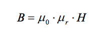
In free space, (i.e. a vacuum devoid of matter) a magnetic field produces magnetic flux according to the following relation.

Where µo is defined as the permeability of free space, and has a value of 4π x 10-7 henrys per meter (H/m). The presence of different materials in a magnetic field will alter the distribution of magnetic flux because they have a magnetic permeability that is different from that of free space. This is discussed further in a later section.

Gauss’ law states that magnetic flux must ‘flow’ in closed loops; flux lines do not terminate on a ‘magnetic charge’. A consequence of this law is that all magnetic fields must exist in the form of dipoles. Every source of magnetic field must have a positive (north) and negative (south) pole. By convention, magnetic flux flows from the source object’s north pole to its south pole outside the object. The magnetic flux returns from the south to the north pole within the object, closing the loop.

Magnetic permeability of materials

When a material is placed in a magnetic field, the magnetic flux density produced in the material is expressed as

Where µr is the relative magnetic permeability of the material. Materials for which µr is less than one are called diamagnetic, since they seem to ‘oppose’ the applied magnetic field. Materials for which µr is greater than one seem to ‘amplify’ the applied field, and are called paramagnetic. Some materials have very high permeability, and these are known as ferromagnetic. All materials that are thought of as being ‘magnetic’ fall in this category.

If the flux density of a vacuum is subtracted from the flux density of a material, the result is a quantity that represents the added flux density due only to the material. This difference can be expressed as µoI where I is the induced magnetization of the material – the magnetic field created by the interaction of the applied field with the material’s magnetic permeability. The total flux density within the material can therefore be expressed as:

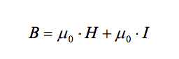
The value I / H is defined as the magnetic susceptibility of the material. Mathematically, this is equal to µr – 1, and it is has no units. Diamagnetic materials will have a negative susceptibility, and paramagnetic materials will have a positive susceptibility. Free space has a susceptibility of 0.

Although susceptibility is unitless, its values differ depending on the system used to quantify magnetic field. This paper will specify susceptibilities in the SI system of units. The cgs system is also commonly used in geology and geophysics. To convert the SI units for susceptibility to cgs, divide by 4π.

Permanent Magnetization

The above section describes the formation of an induced dipole when a magnetic field is applied to a material. When a large magnetic field is applied to a ferromagnetic material and then removed, the material will retain the magnetization that was induced by the high field. This magnetization is known as a permanent dipole. In order to demagnetize a material that has a permanent dipole, a field of opposing direction must be applied to the material. The value of the field that is necessary to demagnetize the material is known as the coercive force, Hc, and is a physical property of the material.

Materials that have a relatively large Hc are known as magnetically hard. Those with a relatively small Hc are known as magnetically soft. This property is not related to the physical hardness of the material.

A ferromagnetic material may also be magnetized (or demagnetized) by heating it above its Curie temperature – by definition the temperature above which the material is no longer paramagnetic. If such a material is cooled in the presence of a magnetic field, it will retain most of the magnetization induced by this field. The permanent magnetization of geological minerals is a result of cooling in the presence of the Earth’s magnetic field.

As a result of this latter effect, most man-made ferromagnetic objects have a permanent magnetization that was introduced when the object was formed. The permanent dipole can be removed from an object by the process of degaussing. Military vehicles are often degaussed by passing them through a suite of magnetometer sensors that can determine the amount of permanent magnetization in the vehicle, and then by applying strong cancellation fields to eliminate the magnetization.

Magnetic Moment 

The concepts of induced and permanent magnetization are not enough to model an object’s total magnetic influence. Magnetic moment is a measure of the total strength of a dipole. Technically, it is defined as the torque experienced when a dipole is at right angles to a magnetic field of unit intensity1 . It is a function of the object’s size and shape as well as its magnetic properties.

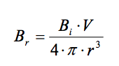
Conceptually, magnetic moment is the integral of the object’s magnetization over its volume. It is also a function of the length of the dipole (the distance between the north and south poles). In order to simplify the calculation of magnetic moment, it is convenient to assume a point-source dipole. This is actually quite accurate if the model need only represent the object’s magnetic influence at distances much farther from the object than the object’s size. In this case, an object’s magnetic moment, M, can be represented by the following relation:

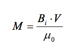
Where Bi is the material’s internal flux density, and V is the material’s volume. M has units of A·m2 . An object’s permanent and induced dipoles will geometrically add to form a single dipole that produces Bi.

Detecting magnetic objects 

Once an object’s magnetic moment is known, one can calculate the intensity of the object’s magnetic influence at varying distances. Conversely, one can use data gathered by a magnetometer to pinpoint the size and location of a magnetic moment of unknown origin. 1 Handbook of Chemistry and Physics 67th ed. CRC Press, 1986. Page F-91. SeaSPY Technical Application Guide rev1.4 Page 4 of 13 Copyright 2007 Marine Magnetics Corp Since the calculative tools described so far by this paper assume that the magnetic moment is generated by a point source, we have as yet no means of using magnetometer data to determine the actual size of an object (i.e. its mass or volume). However, by making a few reasonable assumptions, we can estimate a ferromagnetic object’s size and mass from the size of its magnetic moment.

First, it is very complicated to model the influence of a permanent dipole moment, since it can have any orientation within the Earth’s ambient field, and there is rarely any means to estimate its magnitude. It is therefore convenient to assume a worst-case scenario of no permanent magnetization of the object. Second, the object’s average magnetic susceptibility can usually be estimated with a little bit of information about the material that makes up most of the object. Many man-made structures, especially relatively modern ones, are made of iron-based alloys. For the purposes of this section, we will assume that the object being searched for is made of low-grade, high-carbon iron with a susceptibility of 100. Further information on the susceptibility of iron alloys is available in the next section.

Second, the object’s average magnetic susceptibility can usually be estimated with a little bit of information about the material that makes up most of the object. Many man-made structures, especially relatively modern ones, are made of iron-based alloys. For the purposes of this section, we will assume that the object being searched for is made of low-grade, high-carbon iron with a susceptibility of 100. Further information on the susceptibility of iron alloys is available in the next section.

Our final estimation is that the magnetic influence of a dipole moment is spherical in shape around the dipole’s source. Although this is not precisely true, the amount of error introduced by this estimation will be less than our estimation of the object’s overall susceptibility.

The magnetic influence of a magnetic object can be deduced directly from the object’s dipole moment using the following relation2 :

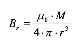
Where Br is the flux density induced by the object at distance r. Using our solution for magnetic moment above, this relation can be expressed as:

The final question that remains is: how can we calculate Bi, the material’s internal flux density? If we go back to the discussion about magnetic permeability of materials, we find that magnetic susceptibility is used to represent the added flux density within a permeable material, over and above that of free space. Bi can be determined by multiplying the material’s susceptibility by the value of the ambient flux density (the intensity of the Earth’s magnetic field at the given location. See the Earth’s Magnetic Field section).

Using the equations given above, we now have the tools we need to estimate the magnetic influence of various sized iron objects at varying distances. The following chart shows the influences of iron objects of different masses, using a density of 7.86g/cm3 . The chart is a log-log plot, which shows the third-order relations as straight lines.

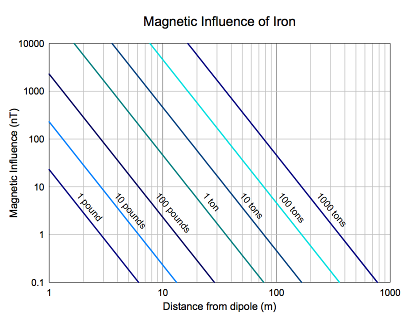
This chart has been calculated assuming no permanent magnetization of the object, a susceptibility of 100, and an ambient field of 50,000nT.

To conclude this section, it must be acknowledged that the above may seem like a lot of approximations. An exacting scientist would have reason to be wary. The assumptions taken here may cause these calculations to be valid only to within an order of magnitude. However, many pieces of information are often not available to the magnetic searcher. Even a coarse approximation such as that offered here is frequently enough to design parameters for a magnetic survey that will be successful in pinpointing the locations of the objects being searched for.

A note about steels and iron alloys 

High purity laboratory-grade iron can have a susceptibility of up to 100,0003 . Alloying elements such as chromium, and impurities such as carbon decrease the susceptibility. In general, high carbon steel and cast iron, although still very magnetic, are less magnetically permeable than low-carbon steels.

Certain types of stainless steel consist of the nonmagnetic austenitic microstructure (an example is marine-grade alloy 316). These steels are rarely used for structural or vehicular applications due to high cost. Welding, machining and cold work of austenitic stainless steel can cause a reversion of the microstructure in the affected area to the more common martensite that is magnetic, making it very difficult to create a practical object from this material that is completely nonmagnetic.

Section 2: Measuring the Earth’s Magnetic Field

The Earth’s Magnetic Field 

The origin of the Earth’s magnetic field is not fully understood, but it is generally accepted that it is caused by electric current generated by movement of the Earth’s conductive, liquid iron-nickel core – a phenomenon known as the dynamo effect. As a result of this effect, the Earth resembles a large rotating permanent magnet.

The magnitude of the Earth’s magnetic field varies from approximately 20,000nT at the southern Brasilian coast to over 65,000nT in northern Canada and Antarctica. The inclination (the angle between the Earth’s field and the horizontal) varies from 90o at the magnetic poles to 0o at approximately the equator.

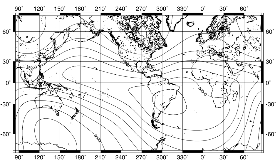
Map of total magnetic field intensity over the surface of the Earth, as of 1995. The contour interval is 5000nT on a Mercator projection. Source: United States Department of Defense.

Diurnal Effects

The magnetic field produced by a single dipole has no distinct boundary; it simply decreases in intensity until it is no longer detectable. The Earth’s field, however, is within the influence of the Sun’s comparatively gigantic magnetic field. The Sun’s larger field interacts with the Earth’s, giving it a distinct boundary. The space within that boundary is known as the magnetosphere. The space outside the magnetosphere is dominated by the Sun’s field, and by a constant stream of free ions and electrons that flows from the Sun, called the solar wind.

Changes in the Sun’s magnetic field affect the Earth’s field dramatically. They continually influence the position of the boundary of the magnetosphere. The Sun’s influence on the magnetosphere is apparent at SeaSPY Technical Application Guide rev1.4 Page 7 of 13 Copyright 2007 Marine Magnetics Corp the Earth’s surface as a low frequency variation that can have high amplitude. Different levels of solar activity can result in changes of several hundred nT in the course of a few hours.

A base station magnetometer (such as Marine Magnetics’ SENTINEL product) is a unit whose sole purpose is to measure diurnal variations, for subsequent correction of mobile survey data. This is a similar concept to using a GPS reference station to correct mobile GPS data. Placing a base station reasonably close to a survey area (within 50-100km) can completely eliminate diurnal effects. Alternately, if increased distance and lower temporal resolution can be tolerated, worldwide magnetic observatory data can be obtained over the Internet from Intermagnet4 .

Total Field and Vector Magnetometers 

Regardless if the source of the anomaly created by a ferromagnetic object is a permanent or induced dipole, or a combination of both, the intensity of the anomaly will always be small when compared with the Earth’s relatively strong ambient magnetic field. When the field of the anomaly is vector-added to the surrounding Earth’s field, the change in the directional component of the Earth’s field will be insignificant. The change in the magnitude of the Earth’s field vector will be far more significant.

Total field magnetometers (like SeaSPY) measure only the magnitude of the magnetic field vector, independent of its direction with respect to the sensor. Vector magnetometers have the ability to measure the component of ambient magnetic field that is projected along one dimension in space. Flux gates, Magnetoresistive, and Hall-Effect sensors are all examples of vector magnetometers.

In order to calculate the total field, three separate vector magnetometer sensors must be oriented at right angles to each other, and their outputs geometrically added by a signal processor. There are practical limitations to how precisely and how rigidly the three sensors can be fixed together at exactly right angles. For this reason, the total-field precision of even the best flux-gate magnetometers is limited to an order of magnitude less than a SeaSPY magnetometer. Furthermore, the output of all vector-field sensors will experience drift with time and with temperature. Vector magnetometers require periodic calibration with an accurate reference such as a proton-spin magnetometer. Proton-spin magnetometers never require calibration, even when first manufactured.

This is why total-field magnetometers are inherently superior to vector magnetometers when the task is detection of ferromagnetic anomalies within the Earth’s magnetosphere, especially for long-term monitoring applications. It is also the reason why total field magnetometers are so widely used in the fields of oceanography, geophysical exploration, and buried object detection.

Section 3: SeaSPY Theory of Operation

Marine Magnetics’ SeaSPY product measures the ambient magnetic field using a specialized branch of Nuclear Magnetic Resonance technology, applied specifically to hydrogen nuclei (protons).

SeaSPY is not what is commonly known as a ‘proton magnetometer’; it is an Overhauser magnetometer. Although still relying on proton spin resonance, an Overhauser magnetometer is as different from a proton magnetometer as a gasoline engine is from a steam engine. Both devices are based on similar physics, but they perform their task completely differently, and this is apparent in their relative levels of performance.

As with steam and gasoline engines, it is important to understand the way a proton magnetometer sensor works before attempting to understand the more sophisticated Overhauser sensor.

Proton-spin magnetometers 

A standard proton-spin magnetometer sensor begins with a small volume of proton-rich fluid such as kerosene or methanol. Inducing a large temporary artificial magnetic field around the liquid (usually with a coil) will cause the spin populations of the protons in the liquid to become biased toward one state, effectively aligning the spin axes of a small majority of protons5 . This is known as polarization. In effect, this process endows the liquid with an induced magnetic moment, since the liquid as a whole behaves as a paramagnetic (or in the case of water, a diamagnetic) material.

When fully polarized (i.e. when the external field has been applied for a long enough time), the proton spin population will follow the following relation:

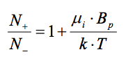
Where N+ and N- are the number of protons with positive and negative spin polarizations respectively, Bp is the ambient (applied) magnetic flux density, and k is Boltzmann’s constant (1.381×10-23 J/K). µi here is the magnetic moment of a proton (1.41×10-26 A·m2 ) – it should not be confused with magnetic permeability.

The larger the ratio of N+ to N-, the larger the overall magnetization of the liquid, and the more signal the magnetometer will be able to produce.

The importance of this relation is that the maximum output signal of a proton magnetometer is proportional to the applied field, Bp. To generate a practical level of signal, Bp must be very large (usually more than 100 times the magnitude of the Earth’s field). This requires a great deal of energy to maintain long enough for polarization to occur.

Once the proton population has been polarized, the proton spin axes are stimulated to precess around the ambient magnetic field vector. This process is known as deflection, since it deflects the proton spin axes from their equilibrium direction with the application of a sharp magnetic pulse. This is analogous to nudging the axis of a spinning top so that it begins to precess around the vertical gravity force vector as it spins.

The alternating magnetic field generated by proton precession may be detected by a coil, and its frequency measured by the magnetometer electronics. This frequency is directly proportional to the magnitude of the ambient field vector.

In practice, the process of polarization and signal measurement are alternated to sample the ambient magnetic field. The proton precession signal cannot be sampled while the polarizing field is in place.

The proton precession frequency will occupy a single narrow spectral line, whose width depends on the chemistry of the solvent. Furthermore, this frequency is completely independent of environmental effects such as temperature. This gives proton-spin total-field magnetometers unsurpassed accuracy and stability characteristics.

The Overhauser Effect

The difference between proton and Overhauser magnetometers is most apparent in the way that the proton spin populations are biased. The Overhauser effect is a phenomenon that uses electron-proton coupling to achieve proton polarization.

A specially engineered chemical that contains a free radical atom6 (an atom with an unbound electron) is added to the proton-rich liquid. The unbound electrons in the fluid can be easily and efficiently stimulated by exposure to low-frequency RF radiation that corresponds to a specific energy level transition. Instead of re-releasing this energy as emitted radiation, the unbound electrons transfer it to nearby protons. This polarizes the protons without the need to generate a large artificial magnetic field.

When polarized, the proton spin population in an Overhauser magnetometer will follow this relation:

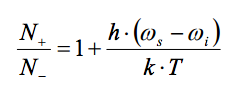
Where h is Plank’s constant (6.626×10-34 J·s), ωi is the proton spin angular frequency, and ωs is the electron spin angular frequency. ωi is a function of the ambient field, and ωs is heavily dependent on the molecular structure of the Overhauser chemical.

The significance of this relation is that the maximum output signal of an Overhauser magnetometer will depend on the design of the Overhauser chemical, not on the amount of energy that is put into the sensor. Consequently, SeaSPY Overhauser magnetometer sensors can produce clear and strong proton precession signals using only 1-2W of power. In contrast, standard proton sensors cannot produce signals that approach the same order of magnitude, even when consuming hundreds of Watts of power.

Another benefit of the Overhauser effect is that polarization power is applied at a frequency that is far out of the bandwidth of the precession signal. Therefore, the sensor can be polarized in tandem with precession signal measurement. This effectively doubles the amount of information available to the magnetometer, allowing faster sampling rates than standard proton magnetometers.

Since Overhauser magnetometers measure the same proton-resonance spectral line as standard proton magnetometers, they exhibit the same excellent accuracy and long-term stability characteristics. Added to this are larger bandwidth, lower power consumption, and sensitivity that is one to two orders of magnitude better.

Section 4: Characteristics of SeaSPY Magnetometers

Magnetometers, like most sensory instruments, consist of two basic parts: a sensor and a measurement device. The sensor produces an analog electrical signal that is proportional to the external influence being sensed, in this case magnetic field. Magnetometer sensors are active sensors, meaning they require external energy to function. The minimum amount of energy required for the magnetometer sensor to do its job is limited by the physics of the magnetometer technology.

The measurement device converts the analog signal produced by the sensor into digital magnetic field units. The measurement device is also frequently responsible for real-time control of the sensor, ensuring that the sensor receives the correct amount of power, or is stimulated properly at the right time.

All total-field magnetometer sensors produce a signal whose frequency is proportional to magnetic field. The measurement device is therefore in essence a very precise frequency counter.

Resolution 

Resolution is a characteristic of the measurement device. It is the minimum change in signal frequency that the measurement device can resolve. In a properly designed device, resolution is reflected by the number of significant digits that are displayed.

SeaSPY’s resolution is 0.001nT, meaning that if an ideal noise-free magnetometer signal were being measured, variations as small as 0.001nT would be detected.

Sensitivity 

Sensitivity is a measure of how small a variation in actual magnetic field can be detected by the instrument as a whole. In a properly designed magnetometer, sensitivity is a characteristic of the sensor, and is a direct function of the base noise level of the sensor signal.

The simplest method of calculating noise level is to assume that the noise within a set of data is broadband (white) noise, i.e. noise that is truly random. If this assumption is true, the root-mean-squared (RMS) model may be applied. The RMS value of a sample of data of n points is represented by the symbol σ. It is calculated as follows:

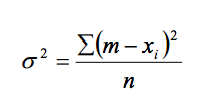
Where m is the mean of the data sample, xi is each data point (from 1 to n), and Σ is the summation operator. σ is also known as the standard deviation of the sample. The units for σ are the same as xi. Therefore the σ of a sample of magnetometer data is represented in nT.

A more accurate method of specifying the noise level of a data set is to divide the noise power in the data by its frequency bandwidth – that is, the entire range of frequencies that the data can possibly represent. The result is called the noise spectral density of the data, and it is represented in units of nT/ √Hz.

The maximum frequency that can be represented by a set of data is one-half the sampling rate, known as the Nyquist frequency. For example, the Nyquist frequency of data sampled at 1Hz is 0.5Hz.

 Bandwidth 

Bandwidth is defined as the range of frequencies of magnetic field variation that can be detected by the magnetometer. SeaSPY’s bandwidth is its Nyquist frequency. Therefore, to calculate the noise spectral density of SeaSPY data sampled at 1Hz, the RMS value of the data sample should be divided by the SeaSPY Technical Application Guide rev1.4 Page 11 of 13 Copyright 2007 Marine Magnetics Corp square root of 0.5. In conditions free of external effects (such as diurnal variation) this value is consistently less than or equal to 0.015nT RMS/√Hz7 .

It should not be taken for granted that a magnetometer’s sampling bandwidth is its Nyquist frequency. One common method for reducing noise is by reducing the amount of high-frequency content in the magnetometer data by applying a digital low-pass filtering algorithm. This technique effectively reduces the sampling bandwidth of the magnetometer.

SeaSPY magnetometers do not apply such a bandwidth-reducing filter to their data. Preserving the maximum possible sampling bandwidth presents the user with as much information as possible, allowing a digital filter to be applied later according to the user’s needs.

Drift 

Drift is the slow change of the magnetometer output with time, without an actual magnetic field change occurring. Drift can be a characteristic of either the sensor or the measuring device. Good design will reduce or even eliminate drift in the measuring device. However, drift in the sensing device usually cannot be reduced by design.

Drift can be best expressed by plotting noise spectral density vs. frequency – i.e. converting the data sample from time domain to frequency domain.

If a data sample is made up of only truly white noise, the frequency spectrum will be ‘flat’. That is, the data set will be made up evenly of all frequencies within the sampling bandwidth of the magnetometer. In contrast, data that exhibits drift with time will show what is known as ‘1 over f noise’, indicating that the noise level increases in the lower frequency area of the bandwidth.

One of SeaSPY’s most powerful features is a complete lack of 1/f noise – a totally flat noise spectrum. This means that a SeaSPY magnetometer is just as sensitive at measuring magnetic field variations as slow as 0.0001 Hz as it is at measuring much faster variations. This characteristic is vital for long-term monitoring, and for creating maps of data that has been collected over long periods of time.

Drift can also appear to occur due to external environmental influences. Temperature drift is the change of the output of the magnetometer as the ambient temperature increases or decreases. A SeaSPY magnetometer will show less than 0.01nT temperature drift over its entire specified temperature range of –40C to +60C. This is because an Overhauser sensor shows no temperature drift, and the SeaSPY electronics measure the sensor frequency using a time reference with extremely high temperature stability.

Heading Error 

Heading Error is a change in the magnetometer’s output that is due to a change in the direction of magnetic field with respect to the magnetometer sensor. There are two possible sources of this effect.

The presence of an induced dipole within detection range of the sensor, and fixed to the tow system, will cause a heading error. This is because the orientation of the dipole will stay parallel to the ambient field. The dipole will therefore change direction with respect to the sensor as the ambient field changes direction with respect to the sensor. Since a dipole’s field of influence is not spherical (see footnote 2) this action will cause a change in the flux density at the sensor’s location.

This source of heading error can be completely eliminated by proper design of the magnetometer as a whole. With sufficient effort, ferromagnetic material can be excluded from all structural components of the instrument. For example, the SeaSPY electronics module contains special custom-made connectors that are made without the layer of nickel that is commonly found underneath gold plating. All of the materials in the SeaSPY towfish, especially those in direct contact with the sensor, are carefully tested to have extremely low magnetic permeability, and are therefore undetectable by the sensor.

The same physics that give SeaSPY Overhauser magnetometer sensors their excellent absolute accuracy characteristics also ensure that the output of these sensors will be completely independent of the ambient magnetic field direction. This is not so for all total-field magnetometers. Some optically pumped magnetometers possess an inherent heading error characteristic that is due to the physics of their operation.

Heading error can be a serious problem. When creating 2-D maps, heading error will show up as an offset between successive survey lines. When searching for small anomalies, this offset can completely obscure potential targets. The heading error offset can be partially compensated for in a 2-D survey by collecting one or more tie lines of data that are perpendicular to the main survey lines. The tie lines can then be used to ‘level’ the main survey data in post-processing. However, it is always more accurate and much simpler to collect heading error-free data to begin with.

Dead Zone

A dead zone is a range of rotation of a total-field magnetometer sensor, with respect to the ambient field, in which the sensor will produce no signal. When this occurs, the magnetometer will not be able to measure the value of the ambient magnetic field.

Some simple proton magnetometer sensors do have a dead zone. This zone is typically a cone along the sensor’s axis that is about ±15o in size. In contrast, SeaSPY Overhauser sensors do not have a dead zone. The amount of signal produced by the sensor is completely independent of magnetic field direction.

Optically pumped total-field magnetometers have a dead zone that is an inherent property of their physics of operation. Unlike an Overhauser sensor, an optically pumped sensor’s dead zone cannot be eliminated by design implementation.

In some applications, a dead zone can be a tolerable shortcoming of a magnetometer. In towed marine applications, however, a dead zone can cause serious operational difficulty. It will restrict the range of headings that the magnetometer can be towed, and will often cause unacceptable complications when towing other instrumentation (such as seismic streamers or side-scan sonar) concurrently. It also makes operation in a remotely operated vehicle (ROV) or an autonomous underwater vehicle (AUV) impractical.

About the Author 

Doug Hrvoic is President and co-founder of Marine Magnetics Corporation. An electrical engineer by profession, he has been designing Overhauser, proton, and optically pumped quantum magnetometers since 1992.

Contact Information 

The purpose of this document is to answer as many questions as possible regarding Marine Magnetics’ SeaSPY magnetometer. It is a work in progress that, it is hoped, will change and grow with time. If you have any questions, suggestions, or information you would like to contribute, please contact us.

References and Further Reading

Craik, Derek. Magnetism – Principles and Applications, John Wiley and Sons, 1995.
A complete investigation of modeling of magnetic sources of all types.

William H. Hayt. Engineering Electromagnetics, 4th ed. McGraw-Hill, 1981.
Chapters 8 and 9 provide a thorough and complete introduction to the first principles of magnetism.

Handbook of Chemistry and Physics, 67th ed. CRC Press, 1986.
Section E119 provides a description and tables of susceptibilities of various materials. Other sections provide a good primer on magnetic properties of materials.

Metals Handbook, desk edition. American Society for Metals Press, 1988.
Section 2-19 describes first principles behind magnetization of materials. Section 20-5 provides a thorough article on materials for permanent magnets

A.P French, Edwin Taylor. An Introduction to Quantum Physics. M.I.T. Press, 1978.
Provides General information on quantum states, and magnetic properties of subatomic particles. Also a good reference for physical constants.

Tom Boyd, Colorado School of Mines. Introduction to Geophysical Exploration. http://www.mines.edu/fs_home/tboyd/GP311/introgp.shtml (web document). An excellent introduction to using magnetometers for geophysical survey purposes. Also describes other useful geophysical survey tools.

Albert Overhauser. Paramagnetic relaxation in metals. Physics Review #89, 1953. pp689-700. In-depth description of the electron-proton coupling phenomenon used in Overhauser sensors. Not related to magnetometry, but interesting reading for the experienced physicist.

J. T. Weaver. Magnetic Variations Associated with Ocean Waves and Swell. Journal of Geophysical Research, vol 70 #8, 1965 Useful knowledge for marine surveyors operating in open water where the size of waves and swell can be significant.