In June 2003, the Naval Undersea Warfare Center (NUWC), Keyport WA, surveyed a small waterway within Puget Sound using a SeaQuest gradiometer system. The goal of the survey was to determine the suitability of the site as a location for the U.S. Navy’s new Electro-Magnetic Field Measurement (EMFM) System, consisting of several stationary magnetic and electric field measurement sensors.

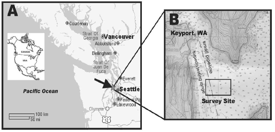
Figure 1: Location of survey site

The purpose of the EMFM system is to measure the relatively small electromagnetic signatures of unmanned undersea vehicles, so selection of a magnetically quiet location was crucial to the success of the project. The area was deemed likely to contain quantities of scrap metal from historical and industrial activities (such as the nearby torpedo testing range) that could interfere with the operation of the EMFM system. The objective of the survey was to locate the geographic position and depth of burial of all ferro-metallic objects within the survey area that would generate anomalies greater than one nanoTesla (nT) and gradients greater than 3 nT/m at a distance of less than 25 m. With that information, the optimum locations for the EMFM System sensors could then be determined.

Figure 2: The SeaQuest three-axis gradiometer system

Marine Magnetics’ SeaQuest system, the only commercially available three component marine gradiometer platform, was chosen for this project since it offers several advantages over total-field sensors and conventional (single axis) magnetic gradiometers. SeaQuest is capable of measuring the transverse, vertical, and longitudinal gradient of the ambient field simultaneously, which allows direct calculation of the Total Magnetic Gradient (a.k.a. Analytic Signal, see Roest et al., 1992) in real time. This greatly reduces post processing time and increases survey accuracy, since the measured total gradient data is free of diurnal variation, as well as immune to the unpredictable effects of permanently magnetized sources and an inclined ambient field. (For a detailed discussion on the threory of total-field gradiometry see the Background Theory section at the conclusion of this document).

Most importantly, the total gradient information enhances near-surface anomalies (such as man-made steel objects) and greatly simplifies the complex three-dimensional information provided by magnetic field data into an easy to interpret form.

The presented results demonstrate the inherent advantages of measuring all three components of the magnetic gradient vector and interpreting total gradient data when attempting to quickly locate the position and depth of ferro-metallic objects. The total gradient data allowed easy identification of several targets in the survey area that otherwise would have been missed by conventional survey methods due to geologically sourced magnetic anomalies.

Instrument Description

The Marine Magnetics SeaQuest system (Figure 2) used in this study consists of a three-sensor biaxial platform that measures transverse horizontal gradient over a baseline of 1.5 m, and vertical gradient over a baseline of 0.5 m. Real-time longitudinal gradient measurement is accomplished by comparing successive total-field measurements to each other using their relative GPS positions along the survey track, or by adding a fourth sensor to the platform tail if higher precision is required. Alternatively the unit may be operated in tandem with a SeaSPY magnetometer for long-baseline measurement. For this study a 3-sensor configuration was used.

SeaQuest’s most important characteristic is the superb absolute accuracy of its Overhauser sensors. If a magnetic gradiometer displays even minute absolute shifts between its sensors, either due to heading effects or systemmatic inaccuracy, it is impossible to correlate adjacent survey lines, and also to relate multiple axis gradient measurements into a single total gradient result (see Equation 1 on page 5). Complex manual adjustment must then be applied post-survey, introducing a major source of error. The SeaQuest system eliminates this error with its Overhauser sensors that are repeatable to better than 0.01 nT, and show zero detectable heading error.

SeaQuest’s Overhauser sensors are also free from ‘dead zones’ which complicate the use of alkali-vapour sensors. Sensors that have a dead zone must be oriented correctly with respect to the inclination of the ambient field in order to produce valid data. This is particularily problematic at mid to low latitudes, where even an optimally oriented sensor will fail to produce data in certain survey line directions.

Another important characteristic is platform stability. Since it is measuring a directional quantity that is heavily dependent on distance from the magnetic source, a gradiometer must provide accurate spatial position data for its sensors. SeaQuest incorporates an acoustic altimeter and pressure sensor to report its vertical position in the water column, and an accurate 2-axis tilt sensor to report pitch and roll. Most importantly, the platform is extremely hydrodynamically stable, which minimizes the need for dynamic compensation for motion effects.

SeaQuest provides a base noise spectral density of 0.01 nT-RMS/rt-Hz per sensor. This translates to roughly 0.009 nT/m noise in horizontal gradient, and 0.028 nT/m noise in vertical gradient. Relating noise levels to actual detectable changes requires us to define a threshold signal-to-noise ratio (SNR) that we can use to identify anomalies. If a SNR of 10 is used to define our minimum detection levels, SeaQuest’s practical magnetic gradient detection levels are 0.1 nT/m horizontal and about 0.25 nT/m vertical. This is an order of magnitude finer than the deviation one would see from gradiometers based on other technologies simply by rotating them in place, and measuring their heading error.

It is important to note that SeaQuest produces raw data that is not filtered – the frequency response extends evenly to the Nyquist frequency, which is the maximum theoretical frequency that data can represent. Filtering the data to a lower bandwidth, a common practice for faster sampling optically pumped magnetometers to reduce the apparent noise level, introduces phase shifts into the data that are different for each frequency being measured. This makes it impossible to correlate signals measured by independent total field sensors, and form an accurate three-dimensional total gradient result.

Survey Parameters

The gradiometer survey was conducted over a two-day period, in addition to side scan sonar and multibeam acquisition. A total of 12 hours survey time were required for the gradiometer.

The survey vessel was a civilian-crewed, wooden-hulled U.S. Navy officer training ship adapted for survey work. SeaQuest was deployed 100 m astern to insure that the magnetic influence of the ship was negligible at the sensor position. The instantaneous depth, altitude, pitch and roll of the tow body were recorded with each magnetic gradient sample.

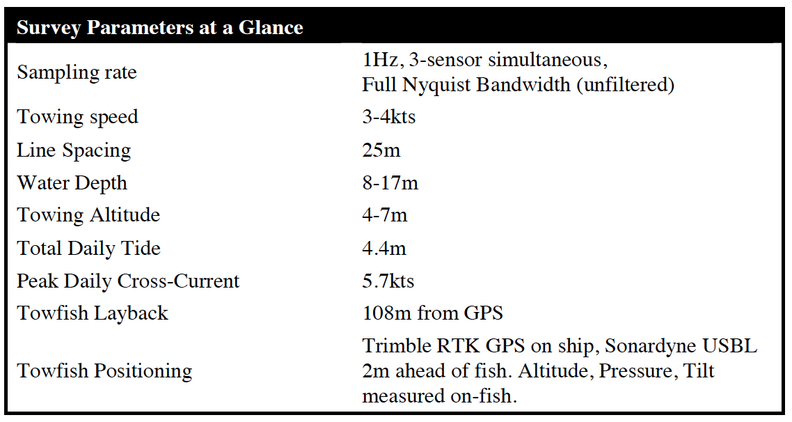
The survey positions were acquired by a Trimble RTK GPS system and adjusted by a Sonardyne USBL transponder. The transponder unit was battery powered, and was mounted on the SeaQuest tow cable 2m forward of the tow body to prevent the transponder’s magnetic effect being measured by the gradiometer. Positioning error was determined to be less than 1m. The adjusted position data was integrated in real time into the SeaQuest data stream by the SeaQuest logging software. Survey lines were created and displayed with QINSy software by QPS.

The survey block consisted of 26 East-West survey lines, nominally spaced at 25m collected in a racetrack fashion over the 650 x 1000m site. Two North-South tie-lines were collected for quality control purposes. In this survey design the measured transverse gradient corresponds to the y-gradient (North-South component of the total gradient) and the longitudinal (along-track) gradient corresponds to the xgradient (East-West component). The vertical gradient is also subsequently referred to as the z-gradient.

The water depth in the survey block varied considerably, with shallow water at the edges and deeper water in the center. A relatively constant pressure depth was used for the bulk of the survey, and vessel speed was increased slightly during line change, allowing SeaQuest to rise over the shallow areas when needed. Figure 3 shows a map of the area bathymetry, calculated with data from the SeaQuest altimeter and pressure sensor. Tide deviation was corrected manually.

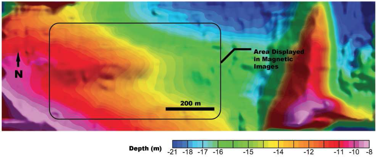
Figure 3: Area Bathymetric Map. Survey lines spanned the entire width and height of the above map, but the ridge to the east was dominated by strong geological magnetism, and was determined to be inappropriate for the Navy’s needs in placement of their AUV-monitoring sensors.

Data Processing

After the survey, the recorded data was imported into Geosoft’s Oasis Montaj software, a package commonly used for professional-quality magnetic data processing and interpretation. As with a typical magnetometer survey, data was evaluated and edited on a line-by-line basis for quality control purposes. Magnetic data was gridded using the minimum curvature method (Briggs, 1977) with a 5m cell size.

Very little processing was required to present the data in the form given in this paper, due in large part to the magnetic cleanliness of the SeaQuest platform, and the high accuracy of the Overhuaser sensors. These characteristics eliminated the need for complex and error-prone filtering and level-shifting operations necessary to obtain usable results with other magnetic gradiometers.

Grids were created directly from measured data only. No compensation for diurnal effect was required, and no heading or altitude compensation was applied. The grids produced were (1)Total field, (2)Xgradient, (3)Y-gradient, (4)Z-gradient and (5)Total-Gradient. The production of the X and Y gradient grids required the data to have the appropriate sign correction applied to account for opposite survey line directions.

The total gradient data (calculated by the SeaQuest acquisition software during the survey), is mathematically equivalent to the Analytic Signal. It is a simple conversion from Cartesian to polar coordinates, and can be described as:

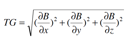
where B is the ambient magnetic field, and dB/dx, dB/dy, and dB/dz are the spatial derivatives (gradients) of the total field in the three Cartesian axes x,y,z. All three of these gradients are measured directly by  SeaQuest, making the calculation of total gradient very simple. This operation reduces the magnetic data to anomalies whose maxima mark the edges of magnetized bodies, as well as centering the anomalies over the source bodies (Roest et al., 1992).

Targets were identified by using the Blakely algorithm (Blakely and Simpson, 1986) to automatically find peaks in the gridded total gradient data. This test compares the values of each grid cell to the values of its neighboring cells. If the current cell has a value higher than all of its adjacent cells it is selected as a target, and its geographic position is recorded to a target list. Targets lists were then separated into primary and secondary based on amplitude of the signal, and interpretation of the other data products.

The apparent depth to the primary targets was calculated by Euler’s homogeneity equation (Euler Deconvolution – Reid et al., 1990) using the produced x, y and z gradient grids from the measured data.

Results

The following pages show the striking contrast between conventional magnetometer (total field) data and the high resolution gradient data obtainable with SeaQuest.

Figure 4 shows the total magnetic field data collected by the top sensor of the SeaQuest platform. This image represents data that would be obtainable by a conventional total field survey and is presented for comparison purposes. The total field image is dominated by north-south trending curvilinear anomalies, which are likely related to magnetic susceptibility variations in the bedrock. This strong background magnetic response makes it difficult to quickly identify anomalies associated with ferrous objects. The amplitudes of these curvilinear anomalies increase eastward suggesting that the depth to bedrock is decreasing eastward. Presenting the total field grid with a ‘stretched’ colour-scale allows identification of at least four potential ferrous targets in the western half of the survey site (arrows).

In contrast, the total gradient map (Figure 5) allows easy identification of at least 12 (high-confidence) ferro-magnetic objects within the survey block. The wavelengths associated with the geological magnetic effects are effectively suppressed in this image in comparison to the total field image. Targets are defined by simple ‘bulls-eye type’ positive anomalies, which are centered over the target position. In the western part of the survey block, a low amplitude NNW-trending linear anomaly is present. This anomaly corresponds to a known pipeline marked on the marine charts of the area. It is worth noting that the amplitude of the pipeline anomaly is less than 0.5nT/m, and yet it is clearly visible in the total gradient map.

Also of interest is the large anomaly slightly to the east of the center of the map. Despite its size, the anomaly is obscured by geology in the total field data, yet it shows up prominently in the total gradient data.

For comparison, the three single-component gradient maps are presented in Figure 6. The data generally shows enhancement of short wavelength anomalies that could define targets. However, interpretation of target positions is still complicated by anomalies that are not centered over the source, anomaly distortion, and remaining geological interference.

It is easy to see that the total gradient (Analytic Signal) directly measured by SeaQuest provides the clearest results, effectively creating an intuituve magnetic ‘image’ of the sea bottom. While the singleaxis gradient results enhance only certain types of anomalies based on their geographic direction, the total gradient is effectively a direction-independent result, enhancing all near-surface anomalies equally, and suppressing deep geology evenly.

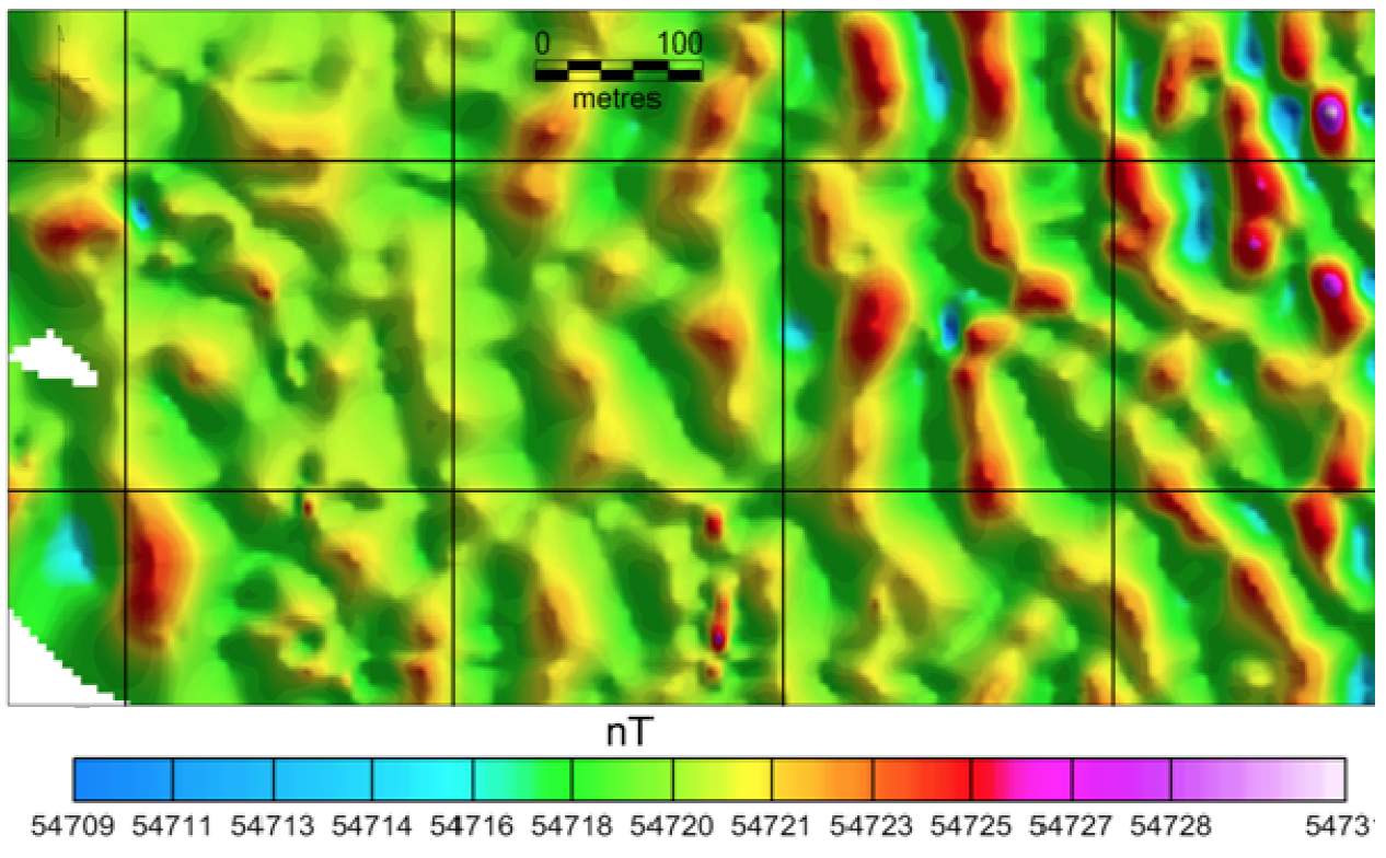
Figure 4: Total magnetic field map of the NUWC survey site. The image is dominated by North-South trending curvilinear anomalies related to buried geology. Only a few ferro-magnetic targets are identifiable (arrows). The Eastern part of the survey block is dominated by geological noise.

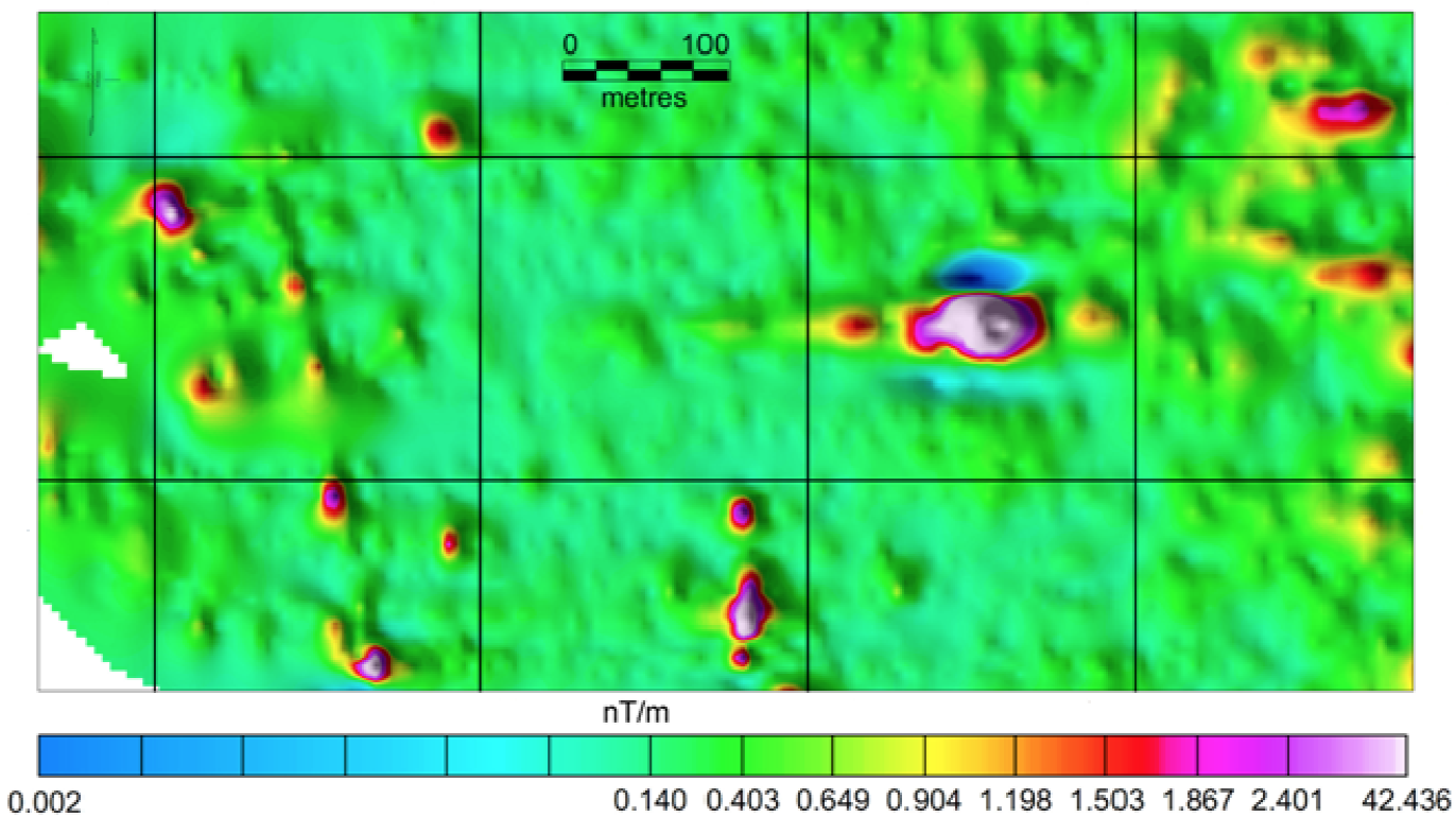
Figure 5: Total Magnetic Gradient (analytic signal) map of the NUWC survey site. The deep geological signal is eliminated, and extremely small targets can be easily resolved, including a faint linear feature in the west that was invisible in the total field data. The linear feature corresponds to a known pipeline.

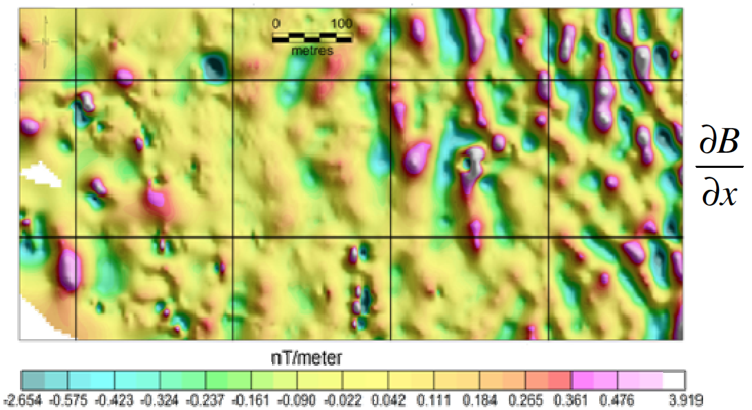
Figure 6: All three measured magnetic gradient axes shown independently. Gradient in the x (East-West) direction. Note enhancement of north-south oriented anomalies. The pipeline in the west of the block is visible, but difficult to interpret.

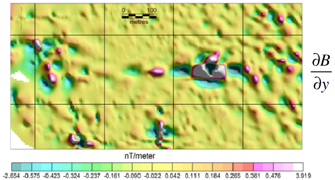
Gradient in the y (North-South) direction. Note enhancement of East-West oriented anomalies. Geology has virtually disappeared because the geological features are N-S trending. However, the pipeline in the west of the block is nearly invisible.

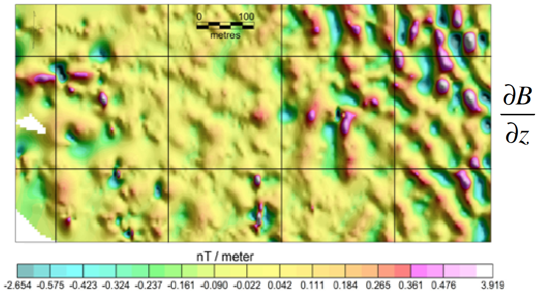
Gradient in the z (vertical) direction. High frequency features are enhanced relatively equally. Note significant remaining influence of the strong deep geology in the east.

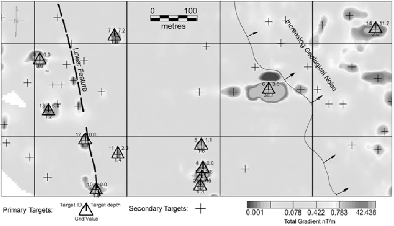
Figure 7: Interpretation of data products overlaid on grayscale total gradient map. Primary target depth estimates (see triangle symbols) obtained from Euler Deconvolution of the measured gradients. Total gradient grid values of the target position provide an estimate of the relative target

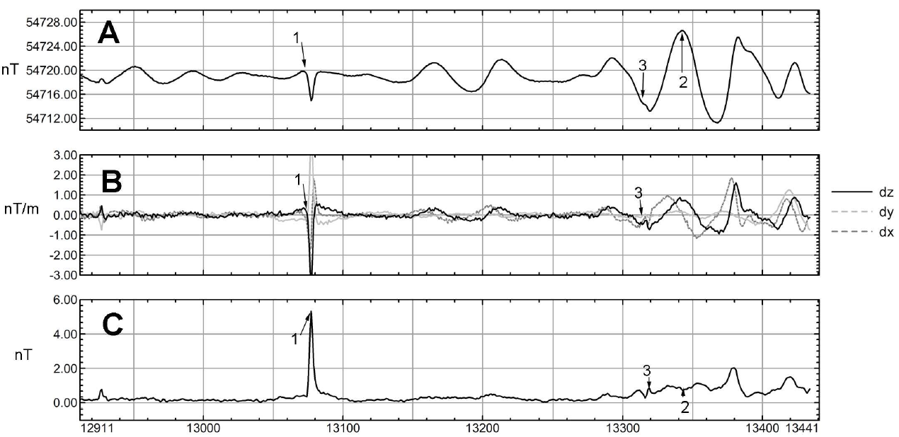
Figure 8: Profile view of one line of SeaQuest data over the NUWC survey site. A- Total-field data recorded from the top sensor. B- Measured x, y and z gradients. C- Corresponding total-gradient calculated in real-time, showing significantly improved signal-to-noise ratio of ferrous targets. Point 1- The complex negative-couplet anomaly measured in the total-field is transformed into a positive peak in the total-gradient, indicating the source position. Point 2- The longer wavelength (deeper) magnetic signal in the total-field profile A is not present in the total-gradient profile C, allowing for easier identification of small near surface targets such as at Point 3.

Conclusions

This paper demonstrates the inherent advantages of directly measuring the Total Magetic Gradient over conventional magnetometer and gradiometer techniques, when searching for small ferro-metallic objects.

Magnetic gradient is commonly used to enhance the signals from small, relatively close sources typical of iron manmade objects, and to suppress the signals from large distant sources associated with geological variation. The total gradient technique goes even further by eliminating the directional dependence of conventional gradiometer methods. This produces an easily interpreted magnetic ‘image’ of the sea floor, with target positions unambiguously marked by ‘bulls-eye’ type anomalies. Also, the total gradient anomalies are expressed with a higher signal-to-background-noise ratio than with conventional techniques, enabling the identification of tiny targets that would otherwise be invisible.

Since the total gradient grid places positive anomalies directly over the source bodies, it allows target maps to be rapidly and accurately generated by an automated peak-picking algorithm, and allows depth estimates to be efficiently obtained by Euler Deconvolution.

The SeaQuest gradiometer platform enables the acquisiton of high-quality total gradient data because of its hydrodynamic stability and the high absolute accuracy of its sensors, producing clean results free from heading errors and offsets. Despite high currents and demanding conditions, SeaQuest provided consistent results that did not require the filtering or level-shifting that are necessary steps, yet large sources of calculation error, for other gradiometer instruments.

What did this mean for the Navy’s goal of placing EMFM sensors for AUV monitoring? SeaQuest revealed a number of magnetic sources that were not detected by acoustic methods, that would have interfered with the Navy’s sensors. The most prominent obstacle was the large anomaly just to the east of the center of the block (Target ID 6 in figure 7).

The Navy’s original goal was to clear the site of magnetic anomalies if any were found. After the survey, divers were sent to investigate several targets, but visibility was zero due to ocean conditions. Further investigation is planned next year.

Instead of clearing the site, the Navy moved its test range to the south-eastern end of the survey block where the gradient data indicated a large magnetically homogeneous area. The EMFM sensors were deployed and are now operating correctly.

Background Theory

Total-field marine magnetometers are routinely used in applications where there is a need to delineate the location and relative size of ferro-metallic objects at or buried below the seabed.

In small target mapping applications using a conventional magnetometer, data is collected on closely spaced survey lines and interpolated into a gridded-array of data cells and displayed as colour-contoured map formats. Targets are located on the map by identifying anomalous short wavelength and comparatively high amplitude deviations in field intensity, which are superimposed on the regional and ‘background’ field variations. In many cases however, the variations in background field may be considerable in comparison to the very small anomalies that define the targets of interest.

Near-surface geologically-sourced magnetic variations and solar-sourced “diurnal” magnetic variations are two examples of problematic ‘background’ magnetic signals. This background noise can mask the targets of interest and thus complicate interpretation. This can lead to missed or falsely identified targets in a survey. The interpretation of magnetic field data at mid to low latitudes is further complicated by an ambient field vector that is inclined with respect to the vertical. This results in dipole anomalies that have a complex waveform (i.e. usually a positive deviation followed by a negative deviation). This makes it less intuitive to determine the exact location of source body. In addition, virtually all man made objects have significant permanent magnetization that can further distort the field variations over a target.

In a conventional magnetometer survey, diurnal variations can be compensated for by the use of a second “base-station” magnetometer. This magnetometer remains stationary for the duration of the survey in order to record the solar-related variations in field intensity so that they can later be removed from the survey data. This correction is essential when the goal of the survey is to produce a high-resolution magnetic map using total-field magnetic data only. However, in marine surveys the use of a base-station magnetometer often complicates the survey logistics and increases costs. For example, finding a suitable location for the base-station, (i.e. that is free of cultural magnetic noise, relatively close to the survey site, and secure enough to leave unattended for a long period of time) can be a major challenge, particularly in urbanized or industrialized locations.

Removing the magnetic effects of geology from survey data is more complex. Often it involves the use of spatial Fourier-domain filters (i.e. upward/downward continuation) applied to the total-field grid to remove the wavelengths in the data associated with the geology (Li and Oldenburg,1998). Several other methods may be successful (i.e. calculation of artificial gradients or the analytic signal from carefully leveled total-field data (Roest et al., 1992). However, all methods require significant processing time and expertise, resulting in increased costs.

Compensation for inclination of the Earth’s field can be carried out by reducing the data to the magnetic pole (Aina, 1986). This filter operation simplifies the vector nature of the field by adjusting the field values to represent data collected in a vertically oriented magnetic field (as at the magnetic pole). This greatly simplifies interpretation, but the process is not stable at low magnetic latitudes (Macleod et al., 1993). Furthermore the process requires the assumption of induced magnetization for all anomalies, which is not valid for almost all ferro-magnetic objects.

Gradiometers

A gradiometer is a specialized type of magnetometer that measures a gradient, or first spatial derivative of the total magnetic field. Gradiometers usually consist of two sensors separated by a fixed distance. The sensors simultaneously measure the total field strength. The difference in measured intensity is divided by the distance between the sensors (baseline distance) resulting in a linear estimate of the gradient of the ambient field. The orientation of the gradiometer will determine what component of the three-dimensional field is measured (usually the x, y, or vertical components).

A well designed magnetic gradiometer has a high degree of immunity from diurnal and magnetic storm activity. Short-baseline magnetic gradient data also shows enhancement of small-wavelength near surface anomalies as generated by ferro-metallic objects, and tends to suppress longer wavelength geological anomalies that may interfere in target mapping applications.

Most commercially available marine gradiometers consist of two synchronized and separated total-field towfish and are limited to measurement of only one gradient component; either the x or y components by transverse or longitudinal configurations. Longitudinal configurations measure the ‘along track’ gradient and consist of the first towfish separated from the second by a length of cable in a ‘single-file’ manner. This gradiometer design is not optimal for target mapping since the separation between the towfish is not rigidly fixed, and thus requires very long baseline distances (i.e. > 20 m) to obtain an accurate gradient measurement.

Transverse marine gradiometers measure the ‘cross-track’ gradient and have the two towfish separated horizontally by a rigid support system, allowing improved resolution of small, near surface anomalies. However, the design has several drawbacks, including the dependency of the survey line direction on the measured gradient direction, and the inability to resolve the vertical component of the gradient vector. In addition, single component gradient data still requires correction for the inclination of the Earth’s field and permanently magnetized sources in order to result in consistent anomalies that are directly over the source bodies.

3-Axis Gradient Measurement

As demonstrated in this study, the measurement of three independent magnetic gradients of the total field using the SeaQuest multiaxis gradiometer system allows real-time calculation of the total-magnetic gradient of the field as described by Equation 1. This operation reduces the magnetic data to anomalies whose maxima mark the edges of magnetized bodies, as well centering the anomalies over the source bodies regardless of the presence of permanent magnetization or inclination of the ambient field. Since the amplitudes in the total gradient grid are derived from a combination of all vector omponents of the field into a simple constant, it can be thought of as a map of total magnetization in the ground.

With the SeaQuest system, gradients are measured as instantaneous observations over short base lines and are thus impervious to diurnal magnetic field effects. The calculated total gradient data is therefore also devoid of diurnal field effects, which eliminates the need for the base-station correction. Due to the frequency of the measured gradients and inherent limitation of the sensitivity of magnetometers, very long wavelength magnetic features are lost in the total gradient information. But this is an advantage in target mapping exercises. Long wavelength information is best viewed by using one or all three of the available total-field measurements.

It is worthwhile to note that data products analogous to the total gradient map in Figure 5 can be produced from single-sensor total field data. It is accepted practice to calculate the Analytic Signal grid, starting with single total field grid (Roest et al., 1992; MacLeod et al., 1993). This process requires calculation of the apparent x, y, and z derivative grids prior to calculation of the analytic signal grid as in Equation 1. However, the results of this process will be vastly inferior to using measured gradient products, and would require a very carefully collected and leveled total field grid in order to create useful results. No matter how good the correction, the results could never approach the quality obtained by the SeaQuest system.

The SeaQuest system employs many design elements to eliminate or reduce as many sources of error in the total gradient as possible. The rigid spacing of the sensors eliminates relative positioning errors. Sensors are extremely accurate and stable so that the measured difference between them will be consistent and repeatable under all conditions. The platform is hydrodynamically stable, maintaining minimal pitch and roll and therefore eliminating errors due to gradient axis orientation.

Authors

Matthew Pozza and Doug Hrvoic of Marine Magnetics Corporation, Richmond Hill Ontario, Canada.

References

Aina, A., 1986, Reduction to equator, reduction to pole and orthogonal reduction of magnetic profiles: Expl. Geophys., Austr. Soc. Expl. Geophys., 17, 141-145.

Briggs, 1974, Machine contouring using minimum curvature. Geophysics, 39, 39-48.

Li, Y. and Oldenburg, D. W., 1998, Separation of regional and residual magnetic field data: Geophysics, 63, 431-439.

MacLeod, I. N., Vierra, S., Chavew, A. C., 1993, Analytic signal and reduction-to-the- pole in the interpretation of total magnetic field data at low magnetic latitudes, Proceedings of the third international congress of the Brazillian society of geophysics.

Reid, A. B., Allsop, J. M., Granser, H., Millett, A. J., Somerton, I. W., 1990, Magnetic interpretation in three dimensions using Euler deconvolution: Geophysics, 55 (1), 80-91.

Roest, W. R., Verhoef, J. and Pilkington, M., 1992, Magnetic interpretation using the 3-D analytic signal : Geophysics, 57, 116-125.

Mapping Marine Ferrous Targets Using the SeaQuest Gradiometer System rev 1.3 Copyright 2011 Marine Magnetics Corp.