
Comparison of a New Marine Magnetometer System to High-Resolution Aeromagnetic Data – A Case Study From Offshore Oman
Brian S. Anderson* (Fugro-LCT), Mark B. Longacre (MBL, Inc.) and Patrick Quist (Fugro-LCT)
Summary
During a marine seismic survey in 1998, conducted offshore Oman for Triton Oman Inc., a marine magnetometer was used to collect a comparison a new magnetic data set for purposes of comparison with a previously flown high-resolution aeromagnetic survey. Profile analysis is provided for purposes of a critical comparison between the two data types.
Introduction
For decades, the standard for towed marine oil exploration magnetometers has been the proton precession technology. Such instruments have proven robust under demanding field conditions, but data has been subject to limitations in resolution due to a combination of measurement technology, external noise sources, and sampling limitations. The Overhauser effect sensor now available to the industry requires lower power, provides dramatically higher signal to noise, and in the configuration tested, provides RS-232 data from the towed sensor, effectively avoiding shipboard noise sources and data “line loss” associated with transmission of small analog voltages from proton precession sensors.
Additional emphasis has been placed on towed marine magnetic data acquisition due to the increased safety of this method when compared to low-level aeromagnetic data acquisition.
Theory of Operation
The Overhauser effect is a phenomenon that dramatically improves the efficiency of a proton magnetometer sensor. Overhauser sensors contain a precisely engineered chemical additive that allows the sensor to be activated or polarized with tuned high frequency radiation. The result is an order of magnitude lower operating power, and one to two orders of magnitude better sensitivity over a standard proton sensor.
Overhauser sensors as illustrated in this case study are also designed to deliver very high absolute accuracy, eliminating drift, heading error, and orientation problems. This characteristic is essential for creating large maps over a long period of time.
Examples from Offshore Oman
The following illustrations are from the offshore Oman case study. Figure 1 illustrates the field area of the survey, with the aeromagnetic data grid shown with an overlay of the 2D marine magnetic survey lines. Figures 2 to 5 are profile comparisons of data. Additional comparisons and vertical continuation comparisons of the data are included in the poster presentation.
The area was an exceptional selection for the data comparison, since the local magnetic field contains a broad spectrum of anomaly amplitudes and wavelengths. Geologically, the Northwestern half of the area is primarily a thick carbonate section, which transitions into an ophiolite field in the Southeastern half of the survey area.
Typical magnetic susceptibility values for carbonate rocks are on the order of 10-6 cgs units, with ophiolites ranging from 10-2 to 10-6 cgs units. These values may vary by an order of magnitude or more in most cases 1,2 .
Description of data (aeromagnetic data):
- Contractor – World Geoscience Corporation
- Diurnally and IGRF corrected, and leveled
- Data every 8 meters along line
- Cesium vapor magnetometer sensor
- Cessna 404 aircraft
- XYZ grid 50 x 50 m, dropped onto lines for comparison
- Flight elevation 80 meters above mean sea level
Description of data (marine data):
- Contractor – LCT
- Tow offset and IGRF corrected
- SeaSPY Overhauser effect magnetometer system
- Resolution 0.001 nT
- Sensitivity 0.015 nT
- Absolute accuracy 0.2 nT
- Approx. 70 meter seismic survey vessel
- Tow distance 300 meters
- Acquired over 19 lines during a 6 day period
- Data every 3 meters along line (1 Hz recording)
- Data not leveled or diurnally corrected
Airborne vs. Marine Magnetometer Comparison – Anderson, Longacre, and Quist
General:
- The resampling of the aeromagnetic data from the final processed grid onto the same projected lines as the marine ship tracks for comparison purposes will be equivalent to the application of a small filter to the aeromagnetic data. Other than this grid to profile operation, no other filtering or operators were applied to the aeromagnetic data used for the comparison, as provided by the Operator
- Two different filters were applied to the marine magnetic data for best comparison with the aeromagnetic data. The initial comparisons are displayed with a 240 second filter on the marine data, and the upward continuation of the marine data was done on data with only a 60 second filter. These filters were applied in order to suppress high frequency low amplitude noise from the movement of sea waves (an electrolyte) over the marine magnetometer sensor.
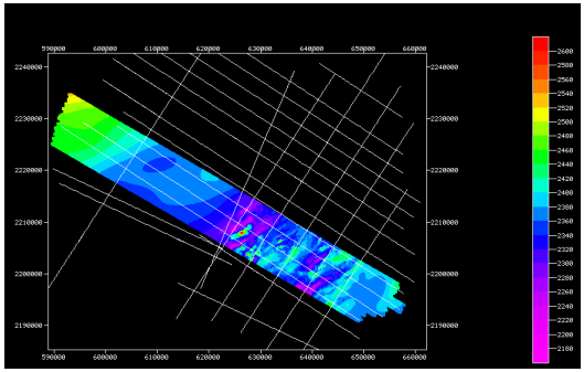
Figure 1: Area of the case study offshore Oman, illustrating the aeromagnetic survey data coverage with an overlay showing the marine magnetometer lines. Note the varied spectral content in the magnetic data, ranging from low to high frequency and low to high amplitude magnetic anomalies.
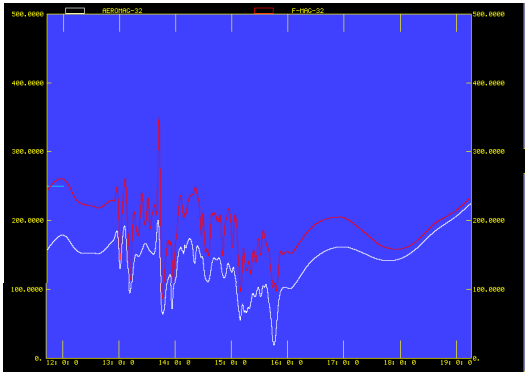
Figure 2: Profile comparison of aeromagnetic data profile extracted from grid (white) vs. marine data (red). A 240 second filter was applied to only the marine magnetometer data. Survey line number 32. Total horizontal scale is 50 kms, total vertical scale is 500 nT.

Figure 3: Zoom in profile comparison of aeromagnetic data profile extracted from grid (white) vs. marine magnetic data (red). A 240 second filter was applied to only the marine magnetometer data. Survey line number 32. Total horizontal scale is 15 kms, total vertical scale is 500 nT.
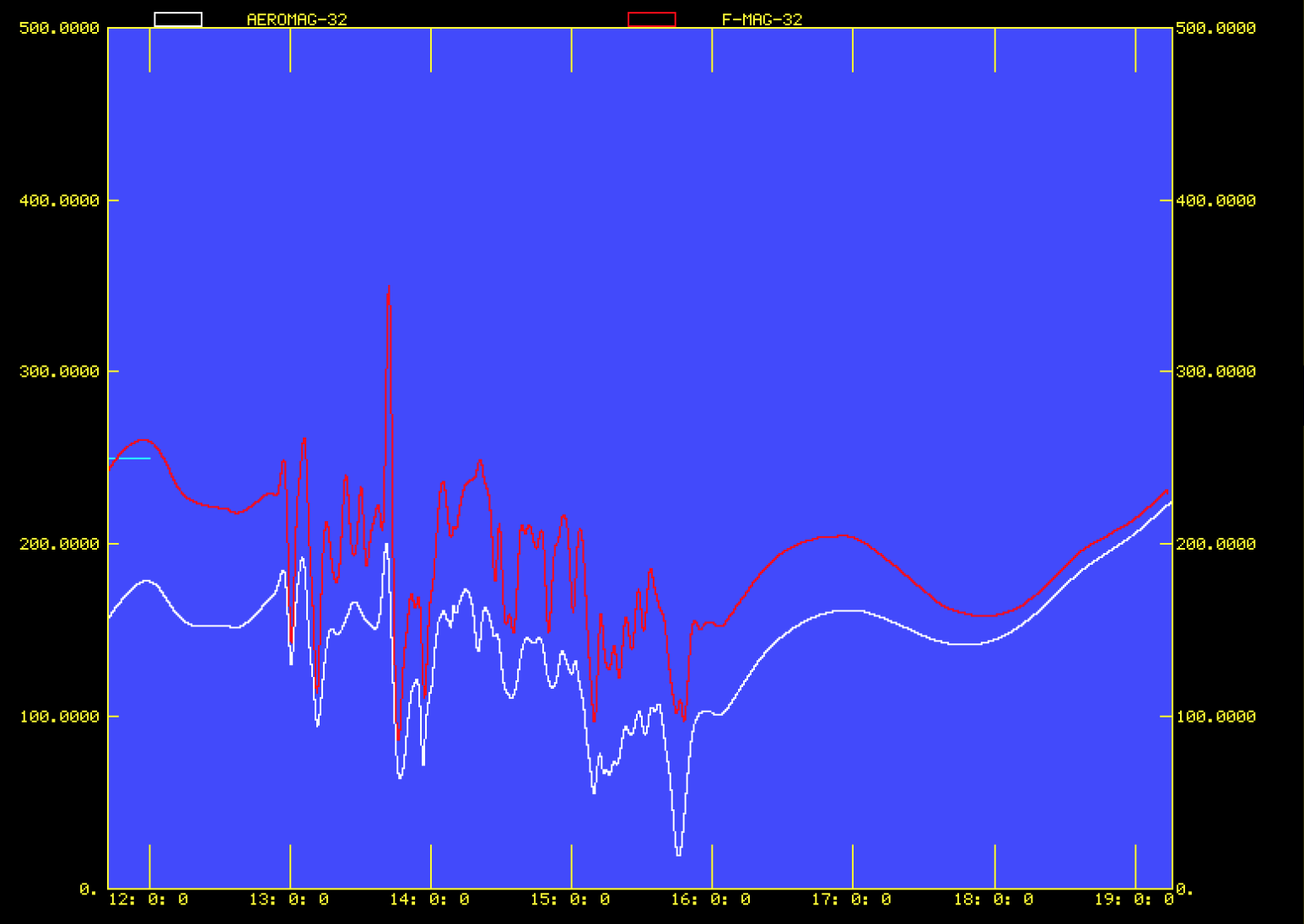
Figure 4: Profile comparison of aeromagnetic data profile extracted from grid (white) vs. marine magnetic data (red). A 60 second filter was applied to only the marine magnetometer data, which has been upward continued 80 meters for comparison purposes. Survey line number 32. Total horizontal scale is 15 kms, total vertical scale is 500 nT.
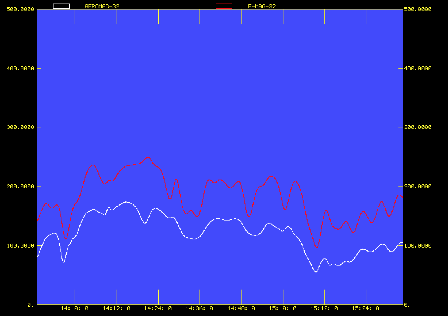
Figure 5: Zoom in profile comparison of aeromagnetic data profile extracted from grid (white) vs. marine magnetic data (red). A 60 second filter was applied to only the marine magnetometer data, which has been upward continued 80 meters for comparison purposes. Survey line number 32. Total horizontal scale is 15 kms, total vertical scale is 500 nT.
Conclusions
This case study illustrates the field performance of the Overhauser effect marine magnetometer system in a real exploration ennvironment. Subsequent field studies have shown similar system performance in other areas of the world.
In comparison with vintage marine magnetometer data, the Overhauser system is providing an order of magnitude higher resolution marine magnetic data than the industry has consistently achieved with other technologies. These improvements, in parallel with lowered risk to data acquisition personnel, provide significant advances in the state of the art for marine magnetic mapping.
Acknowledgements
The authors would like to thankfully acknowledge The Management of Triton Oman, Inc. and the Oman Ministry of Oil and Gas for their providing access to the data presented.
References
1. S. Breiner, Applications Manual for Portable Magnetometers, Geometrics Publication, 1973.
2. L. Nettleton
Brown, R.P., Comeaux, L.B., and Ward, R.W., Submitting an Expanded Abstract Using sSubmit, Society of Exploration Geophysicists International Exposition and 68th Annual Meeting, New Orleans 1998.
Ross, C.P. and Verm, R.W., Submitting an Expanded Abstract Using Submit with EASE, Society of Exploration Geophysicists International Exposition and 69th Annual Meeting, Houston 1999.